

Updated: August 16, 2026
OPRS may receive compensation when readers open an account through partner links on this page. Our analysis is based on independent research, BBB data, and IRS publications.
The single strongest predictor of a retiree selling equities at the bottom of a bear market is not risk tolerance measured on an intake form. It is the number of months of spending sitting in cash on the day the market drops. A retiree who sees two years of grocery money already parked in Treasury bills does not need to sell stocks in March 2020, or in October 2022, or in any other panic window.
That single behavioral fact is the point of the bucket strategy. It does not change expected return in a meaningful way. It changes the odds that the retiree stays invested long enough to earn the return the market offers. This page walks through the mechanics of the classic three-bucket design, a labeled worked example, the refill logic, and the honest critiques.
Origin: Harold Evensky and the 1996 Wealth Management book
The three-bucket approach was popularized by Harold Evensky, a Florida-based certified financial planner, in his 1996 book Wealth Management. Evensky called it a cash-flow reserve strategy. The idea was to hold a defined amount of near-cash so that daily and annual living expenses did not depend on the closing price of the equity portfolio.
Evensky argued that the reserve was worth its lower expected return because it kept the retiree from being forced to sell risk assets during a downturn. Later planners generalized the idea into two or three buckets, each pinned to a spending horizon. The label bucket strategy stuck. The mechanics have not changed much since.
The three buckets defined
The canonical version uses three time-segmented pots. Each pot is sized against a specific window of retirement spending. Instruments inside each pot match the risk that the pot is expected to bear over that window.
- Bucket 1: short-term, years 1 and 2. Cash in an FDIC-insured savings account, a money-market fund holding short Treasury bills, or laddered T-bills maturing inside twenty-four months. Zero equity exposure. This is the pot the retiree draws from for groceries, utilities, and health premiums.
- Bucket 2: medium-term, years 3 through 10. Intermediate high-quality bonds and short-to-intermediate bond funds. Enough duration to earn a real yield above cash, short enough that a rate shock does not drop the pot by more than a few percent.
- Bucket 3: long-term, years 11 and beyond. A diversified stock and long-bond portfolio. This pot is expected to see full equity volatility. It is also the pot expected to grow real spending power over a twenty- or thirty-year retirement.
The exact percentages are not the point. Two years of spending is a common floor for bucket 1 because most historical US bear markets have recovered inside twenty-four months. Beyond that, sizing depends on the household spending plan, other income sources, and the retiree’s tolerance for seeing bucket 3 fall in value.
A labeled worked example: a $600,000 portfolio
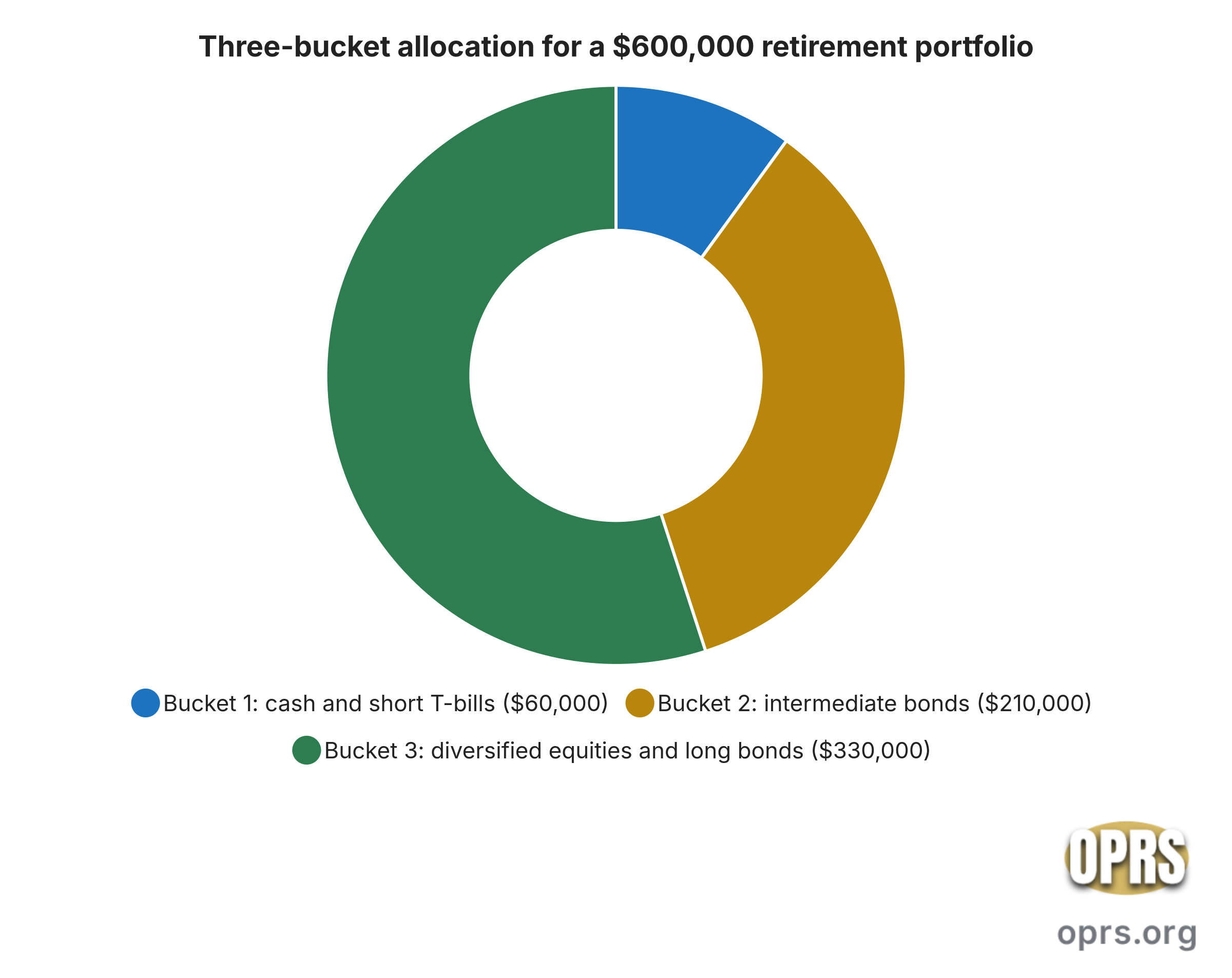
Assume a retiree with $600,000 in a rollover IRA and a planned withdrawal of $30,000 per year in today’s dollars, layered on top of Social Security. That $30,000 anchor sets the size of each bucket. The three pots below are one common allocation, not the only defensible one.
- Bucket 1, cash and short Treasury bills: $60,000 (two years of the $30,000 draw).
- Bucket 2, intermediate investment-grade bonds: $210,000 (roughly seven years of draw, filling out years three through nine).
- Bucket 3, diversified equities and long bonds: $330,000 (year ten and beyond, expected to grow in real terms).
The percentage split is 10 percent cash, 35 percent bonds, and 55 percent equities. That looks conservative next to a traditional 60-40 portfolio and aggressive next to a laddered-bond-only design. It is a middle path that most academic simulations rate as broadly comparable to a static 60-40 in long-run outcome.
The refill logic: how buckets replenish
The strategy only works if bucket 1 gets refilled on a rules-based cadence. Otherwise the retiree spends down cash, discovers year three is coming, and either sells bonds at a bad price or panics into equities at the wrong moment. Refill rules turn the design into a discipline instead of a hope.
- Annual harvest, rules-based. Once a year, if bucket 3 is up by a defined threshold (some planners use plus 5 or plus 10 percent for the calendar year), sell enough equities to refill bucket 2 back to its target size. Then move one year of spending from bucket 2 into bucket 1.
- Defer if stocks are down. If bucket 3 finished the year flat or negative, skip the equity harvest. Refill bucket 1 by drawing from bucket 2 only. Bucket 3 gets left alone to recover.
- Interest and dividend sweep. Interest paid inside bucket 2 and dividends paid inside bucket 3 usually route to bucket 1 by default, cushioning the annual draw even in flat markets.
- Rebalance around the refill. The refill itself is a rebalance. It naturally trims the pot that grew fastest and adds to the pot that got drained.
Some households formalize the rule further. A one-page written policy usually reads like this. Refill bucket 1 to twenty-four months every February. Refill bucket 2 by selling equities only if the S&P 500 is above its level twelve months earlier. Otherwise draw from bucket 2 and wait.
Why the strategy is fundamentally behavioral
The academic critique of the bucket strategy, restated below, is that once you flatten the three pots you get a lifecycle allocation not far from a plain 60-40 or 55-45. In pure expected-return terms the two designs are close. The bucket strategy is not selling more math than a static allocation.
What it does sell is a mental frame. A retiree who can point to two years of Treasury bills and eight years of investment-grade bonds does not need bucket 3 to be flat this year. That single sentence is worth more than any Monte Carlo output when the market drops 30 percent in a month.
Studies of retiree behavior during 2008 and 2020 consistently found that the households most likely to sell equities at the bottom were the ones with no explicit cash reserve. Households with a defined near-cash pot were far more likely to stay the course. That behavioral gap, not the allocation gap, is the return the bucket strategy earns.
Comparison to the systematic-withdrawal approach
The systematic-withdrawal approach starts from a static allocation (often 60-40) and takes the annual draw pro-rata from all holdings. It is simpler to run and easier to model. It also asks the retiree to sell equities in the same month a headline calls the market a lost decade.
Purely on expected return, the two designs finish close. The bucket strategy costs a small amount of drag because bucket 1 earns less than the market. In exchange it buys a defined runway of spending independent of the equity print. For a household that has watched a spouse or parent sell at the bottom once, the drag is a fair price.
Interaction with sequence-of-returns risk
The bucket strategy is a direct response to sequence-of-returns risk: the risk that a large loss in the first few years of retirement permanently reduces the portfolio’s ability to fund the plan. A retiree drawing $30,000 from a $600,000 portfolio that then drops 30 percent is in a different plan than a retiree whose portfolio dropped 30 percent in year fifteen.
Bucket 1 and bucket 2 exist so the retiree does not need to sell into that early loss. The refill rule locks in the defer-if-down logic. Together they neutralize much of the sequence risk that a static allocation carries. The mechanics of sequence risk itself, and why it hits early retirees hardest, are covered in the OPRS reference on sequence-of-returns risk for early retirees.
Social Security and pensions as an implicit bucket 0
Any inflation-linked lifetime income the household already receives acts as an implicit bucket 0 that sits below the three portfolio buckets. Social Security, a defined-benefit pension, and an inflation-adjusted annuity all fall in this category. The Consumer Financial Protection Bureau’s before-you-claim tool is a plain-language starting point on how the Social Security piece interacts with a retiree’s spending floor.
The larger this implicit floor, the smaller bucket 1 and bucket 2 need to be. A household with $40,000 of combined Social Security and pension against $50,000 of spending only needs the portfolio to cover a $10,000 gap. The bucket sizing collapses in proportion. The math is easier and the required equity allocation can be lower without sacrificing lifestyle.
The reverse is also true. A retiree who claims Social Security very early and gets a smaller monthly benefit is asking bucket 3 to work harder for longer. That is not a reason to avoid claiming early, but it is a reason to size bucket 1 with the actual claiming decision in mind, not the estimate at full retirement age.
Pairing with the 4 percent rule and guardrails methods
The 4 percent rule sets the initial withdrawal rate. The bucket strategy sets where the money comes from. The two answer different questions and can be run together.
A common combined policy: use the 4 percent rule to size the year-one draw (4 percent of the day-one portfolio), then adjust that draw for inflation each year. Use the three-bucket structure to source the draw. The 4 percent rule tells the retiree how much to take. The buckets tell the retiree which pot to take it from.
Guardrails methods (Guyton-Klinger and its cousins) add a second layer: if the withdrawal rate drifts above or below defined bands, cut or increase the draw. Guardrails and buckets combine well. Guardrails control the size of the draw. Buckets control the timing of the sales that fund it.
Honest critiques
Three critiques of the bucket strategy are well-founded and worth naming outright.
- Mental accounting fallacy. Money is fungible. Labeling one dollar as bucket 1 and another as bucket 3 does not change the aggregate risk of the portfolio. Academics such as Michael Kitces have shown that a flattened three-bucket allocation often looks a lot like a static 55-45 or 60-40 in aggregate.
- Cash drag in placid markets. In a decade with steady equity gains and no major drawdown, bucket 1 earns less than the market and drags total return. That drag is real. It buys behavioral insurance the retiree may not need in that specific decade, but cannot know in advance.
- Refill discipline is hard. Written refill rules require the retiree, or an advisor, to actually run them. Households that abandon the refill logic after the first bear market end up with a top-heavy allocation right when they need the reverse.
None of the three critiques kill the strategy. They set the expectation that the bucket approach is a behavioral tool sitting on top of the same fundamentals every other retirement-income plan uses. The gain is real, the cost is real, and both are visible at design time.
Sources cited
- U.S. Securities and Exchange Commission, Investor.gov, Investment Products overview, covering the cash-equivalent, bond, and equity instrument categories that populate each bucket in a time-segmented retirement plan.
- Consumer Financial Protection Bureau, Planning for Retirement: Before You Claim, an interactive tool that shows how Social Security claiming age changes the monthly benefit that functions as the household’s implicit bucket 0 income floor.
- FINRA, Investors: Investment Accounts, Retirement Accounts overview, describing the tax-advantaged account wrappers (Traditional IRA, Roth IRA, 401(k), 403(b), TSP) inside which the three-bucket allocation is typically implemented.